Note
Go to the end to download the full example code.
Module efficiency models#
Fit seven models to sample measurements and find the best one.
from pvpltools.module_efficiency import (
    adr,
    heydenreich,
    motherpv,
    pvgis,
    mpm5,
    mpm6,
    bilinear,
)
from pvpltools.module_efficiency import fit_efficiency_model, fit_bilinear

import numpy as np
import pandas as pd
import matplotlib
import matplotlib.pyplot as plt

from pathlib import Path
import os

# different current working directories for Sphinx-gallery / normal interpreter
try:
    cwd = os.path.dirname(__file__)
except NameError:
    cwd = os.getcwd()
cwd = Path(cwd)

matplotlib.style.use("classic")
matplotlib.rcParams["figure.facecolor"] = "w"
matplotlib.rcParams["axes.grid"] = True
matplotlib.rcParams["lines.linewidth"] = 2
Now get some efficiency measurements to work with. A file containing module matrix measurements can be downloaded from the PVPMC website at https://pvpmc.sandia.gov/download/7701/.
# this is the filename of the data file under "examples/data"
measurements_file = cwd.parent.joinpath(
    "data", "Sandia_PV_Module_P-Matrix-and-TempCo-Data_2019.xlsx"
)

# The first sheet is for the Panasonic HIT module
TYPE = "Panasonic HIT"

matrix = pd.read_excel(
    measurements_file,
    sheet_name=0,
    usecols="B,C,H",
    header=None,
    skiprows=5,
    nrows=27,
)
matrix.columns = ["temperature", "irradiance", "p_mp"]

# calculate efficiency from power
matrix = matrix.eval("eta = p_mp / irradiance")
eta_stc = matrix.query("irradiance == 1000 and temperature == 25").eta
matrix.eta /= eta_stc.values

# just keep the columns that are needed
matrix = matrix[["irradiance", "temperature", "eta"]]

matrix
it really is matrix data this becomes more obvious when you pivot it
grid = matrix.pivot(index="irradiance", columns="temperature", values="eta")

grid
now fit my favorite model
popt, pcov = fit_efficiency_model(
    matrix.irradiance,
    matrix.temperature,
    matrix.eta,
    adr,
)
popt
array([ 0.99879112, -5.85209308, 0.01939665, 0.0696307 , 0.21036569])
wait, it can’t be that easy!
adr(600, 15, *popt)
np.float64(1.022515949060066)
yes it can
define some ranges for plotting
ggg = np.logspace(-0.1, 3.1, 51)
tt = np.array([0, 15, 25, 50, 75, 90])
Plot the results
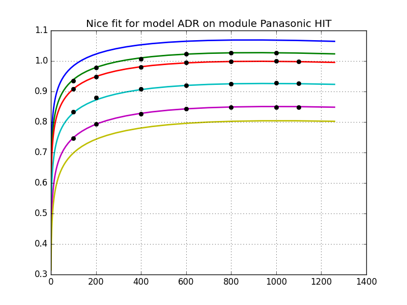
Text(0.5, 1.0, 'Nice fit for model ADR on module Panasonic HIT')
Gather plotting commands into a convenient function
def plot_model(model, params):

    ggg = np.logspace(-0.1, 3.1, 51)
    tt = np.array([0, 15, 25, 50, 75, 90])

    plt.figure()
    plt.gca().set_prop_cycle(
        "color", plt.cm.rainbow(np.linspace(0, 1, len(tt)))
    )

    for t in tt:
        plt.plot(ggg, model(ggg, t, *params))

    plt.xlim(-50, 1350)
    plt.ylim(0.45, 1.15)
    plt.xlabel("Irradiance [W/m²]")
    plt.ylabel("Relative efficiency")
    plt.legend(tt, title="Temperature", ncol=2, loc="best")
    plt.title(model.__name__.upper())
    return plt.gca()


ax = plot_model(adr, popt)
ax.plot(grid, "ko")
[<matplotlib.lines.Line2D object at 0x7fa8c2bc1f40>, <matplotlib.lines.Line2D object at 0x7fa8c2cba900>, <matplotlib.lines.Line2D object at 0x7fa8c2bc1dc0>, <matplotlib.lines.Line2D object at 0x7fa8c2c9ee40>]
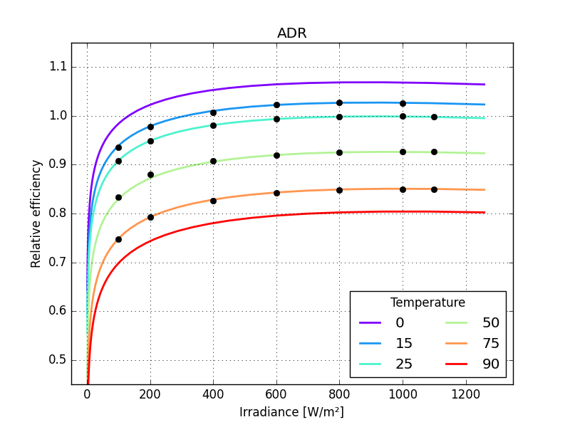
now run and plot all the available models


make a function to calculate rms error
def efficiency_model_rmse(irradiance, temperature, eta, model, p):

    from numpy import sqrt as root, mean, square

    eta_hat = model(irradiance, temperature, *p)

    return root(mean(square(eta_hat - eta)))


rmse = efficiency_model_rmse(
    matrix.irradiance, matrix.temperature, matrix.eta, model, popt
)

print(TYPE, model.__name__.upper(), rmse)
Panasonic HIT ADR 0.002028199009144769
compare the models
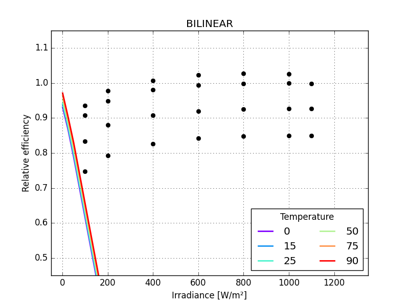
Panasonic HIT, BILINEAR 2.30300
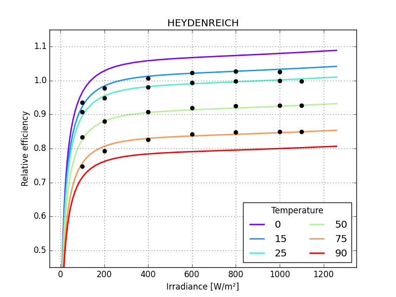
Panasonic HIT, HEYDENREICH 0.00605
Panasonic HIT, MOTHERPV 0.00249
Panasonic HIT, PVGIS 0.00158
Panasonic HIT, MPM5 0.00291
Panasonic HIT, MPM6 0.00279
Panasonic HIT, ADR 0.00203
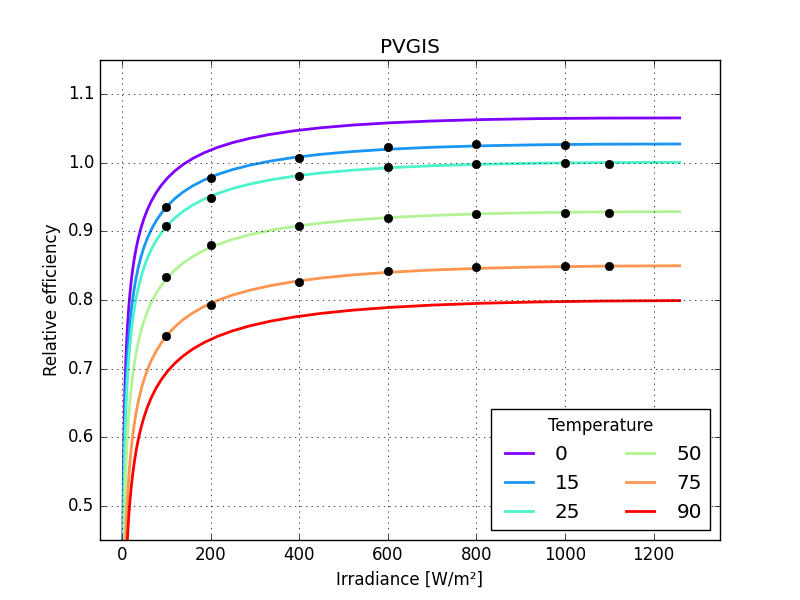
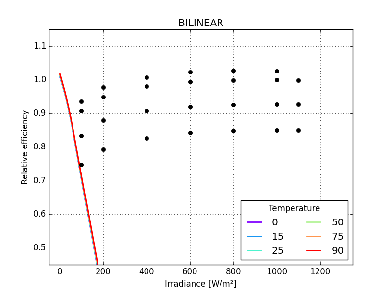
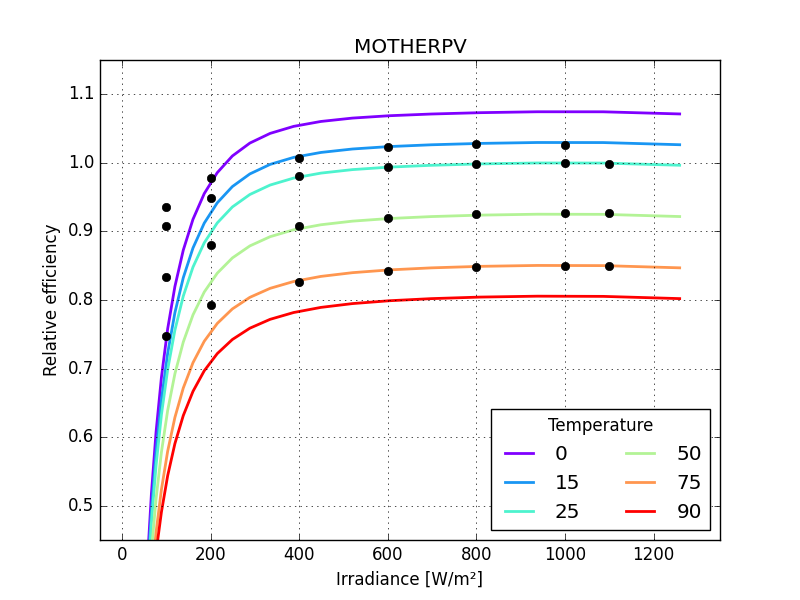
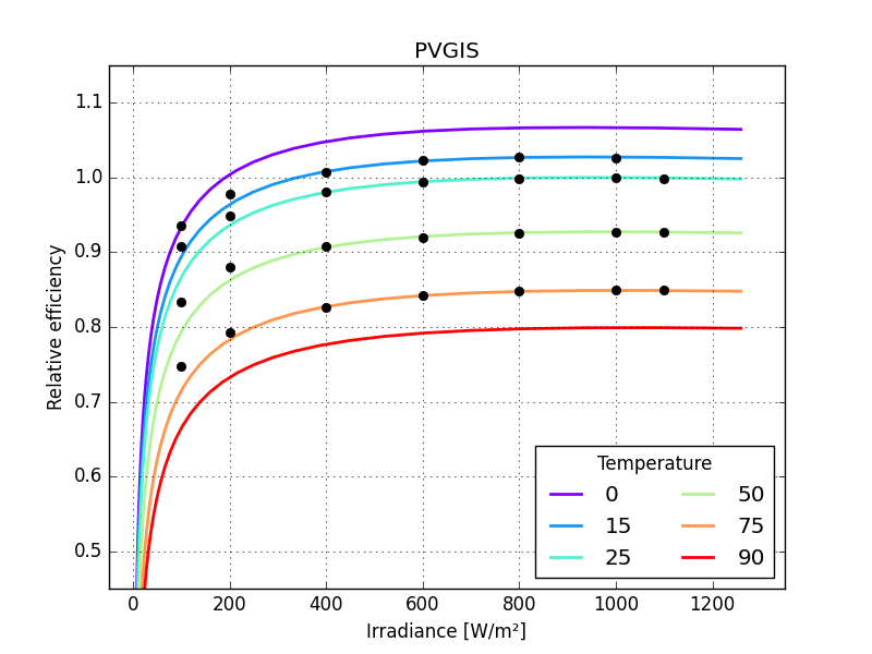
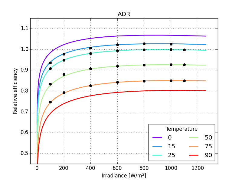
now run one of the harder tests: extrapolating to the low irradiance values
subset_fit = matrix.query("irradiance >  200")
subset_err = matrix.query("irradiance <= 200")

for model in models:

    if model is bilinear:
        interpolator = fit_bilinear(**subset_fit)
        popt = [interpolator]
    else:
        popt, pcov = fit_efficiency_model(**subset_fit, model=model)

    rmse = efficiency_model_rmse(**subset_err, model=model, p=popt)

    print("%20s, %-20s %.5f" % (TYPE, model.__name__.upper(), rmse))
Panasonic HIT, BILINEAR 0.40747
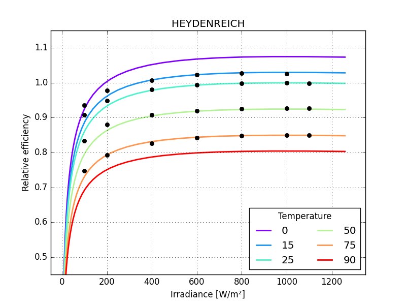
Panasonic HIT, HEYDENREICH 0.02965
Panasonic HIT, MOTHERPV 0.15097
Panasonic HIT, PVGIS 0.02889
Panasonic HIT, MPM5 0.00490
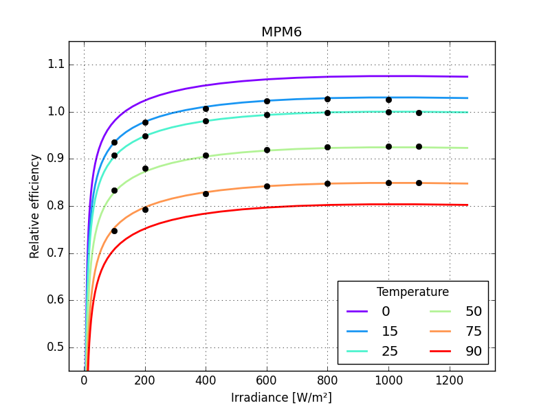
Panasonic HIT, MPM6 0.08156
Panasonic HIT, ADR 0.00401
the graphs make these differences more striking
for model in models:

    if model is bilinear:
        interpolator = fit_bilinear(**subset_fit)
        popt = [interpolator]
    else:
        popt, pcov = fit_efficiency_model(**subset_fit, model=model)
    plot_model(model, popt)
    plt.plot(grid, "ko")

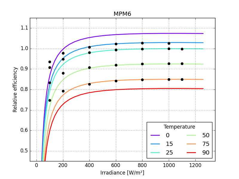
just one small detail missing: the last parameter of MPM6 should not be larger than zero so bounds need to be defined for all its parameters
MPM6_BOUNDS = (
    [
        -np.inf,
        -np.inf,
        -np.inf,
        -np.inf,
        -np.inf,
    ],
    [+np.inf, +np.inf, +np.inf, +np.inf, 0.0],
)

model = mpm6

popt, pcov = fit_efficiency_model(
    **subset_fit, model=model, bounds=MPM6_BOUNDS
)
rmse = efficiency_model_rmse(**subset_err, model=model, p=popt)

print("%-20s %-20s RMSE = %.5f" % (TYPE, model.__name__.upper(), rmse))
print("popt =", popt)
Panasonic HIT        MPM6                 RMSE = 0.08156
popt = [ 1.03574966 -0.00299249 -0.04758015 -0.00717004 -0.0290341 ]
in this case the bounds did not influence the result
Total running time of the script: (0 minutes 1.846 seconds)